
Key Takeaways
- Statistical significance is about chance, not importance: A result is "statistically significant" when the observed effect would be unlikely if the null hypothesis were true (commonly judged by p < 0.05).
- A p-value is not the probability your result is wrong: It is the probability of seeing results at least this extreme assuming the null hypothesis is true.
- Sample size drives significance: Large samples can make tiny differences significant; small samples can miss meaningful effects. Plan sample size before collecting data.
- Always pair significance with effect size: A statistically significant result can be trivially small. Report the magnitude of the difference alongside the p-value.
- Significance testing follows a fixed procedure: State hypotheses, choose alpha, compute a test statistic, obtain a p-value, compare to alpha, and decide.
What statistical significance means
A result is statistically significant when the data provides strong enough evidence that the observed effect is unlikely to be explained by chance alone.
More precisely, statistical significance is a decision rule used in hypothesis testing. Researchers start with a null hypothesis (usually "there is no difference" or "there is no effect") and then ask: if the null hypothesis were true, how surprising would the observed data be? If the answer is "very surprising" (technically: if the p-value falls below a pre-set threshold called alpha), the result is declared statistically significant.
Government and institutional glossaries describe this in the same spirit: statistical significance indicates that an observed result is unlikely to be due to chance alone under a specified model and threshold (see CDC definition and NIH NCATS glossary).
Is: evidence against a specific "no effect" claim (the null hypothesis), given assumptions about the data and test.
Is not: proof your hypothesis is true, proof a result is important, or a guarantee the finding will replicate.
The concept dates back to Ronald Fisher's 1925 work Statistical Methods for Research Workers, which popularized the 0.05 threshold still in wide use today. Fisher treated it as a rough guide, not a rigid rule, but the convention stuck and spread across virtually every empirical discipline.
How significance testing works
Most significance tests follow the same five-step procedure. This is the logic that underlies every z-test, t-test, chi-square test, and ANOVA.
Step 1: State the hypotheses
Null hypothesis (H0): No difference or no effect exists (e.g., "Male and female IQ scores are equal in the population"). Alternative hypothesis (H1): A difference or effect does exist.
Step 2: Choose alpha
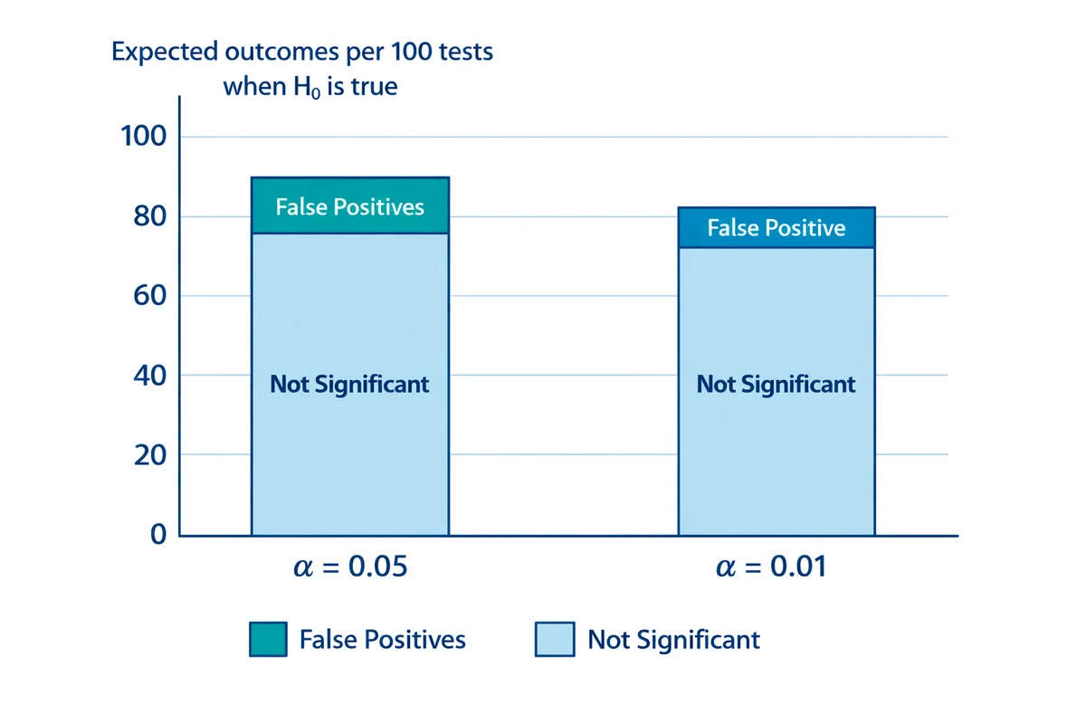
Alpha is the significance level, the threshold for calling a result "significant." The most common choice is alpha = 0.05 (5%). This means you accept a 5% risk of a false positive.
Step 3: Collect data and compute a test statistic
The test statistic (z, t, chi-square, F, etc.) summarizes how far the observed data deviates from what the null hypothesis predicts. Larger values mean more deviation.
Step 4: Find the p-value
The p-value is the probability of getting a test statistic at least as extreme as yours, assuming H0 is true. A small p-value means the data are hard to reconcile with the null hypothesis.
Step 5: Compare p to alpha and decide
If p < alpha, reject H0 and call the result statistically significant. If p ≥ alpha, fail to reject H0. "Fail to reject" is not the same as "accept H0." It means the evidence was not strong enough to rule out chance.
Example: Suppose 1,000 people take an IQ test. The mean score for males is 98 and for females is 100. A two-sample t-test yields p = 0.001. Because 0.001 < 0.05, the difference is statistically significant. But is a 2-point IQ difference meaningful? Almost certainly not. This is the classic illustration of why significance is not the same as importance (more on that in the practical significance section).
If the same 2-point gap appeared in a sample of only 25 people, the t-test would likely return p > 0.05 and the difference would not be significant. The underlying truth did not change, but the evidence (sample size) did. This is why sample size planning matters. For a refresher on how to build the study that feeds this analysis, see questionnaire design principles.
How to interpret p-values
The p-value is the most widely reported (and most widely misunderstood) number in significance testing.
Correct interpretation: A p-value of 0.04 means that if the null hypothesis were true, you would see results as extreme as yours (or more extreme) about 4% of the time due to random sampling variability.
Common misinterpretations to avoid:
- "There is a 4% chance the null hypothesis is true." Wrong. The p-value is calculated under the assumption that H0 is already true. It says nothing about the probability that H0 is true or false.
- "There is a 96% chance the result will replicate." Wrong. Replication probability depends on the true effect size, sample size, and study design, not the p-value alone.
- "The result is important." Wrong. A small p-value means the data are unlikely under H0. Whether the result matters practically is a separate question.
The American Statistical Association addressed these misinterpretations directly in its landmark 2016 statement, noting that "a p-value does not measure the probability that the studied hypothesis is true, or the probability that the data were produced by random chance alone" (Wasserstein & Lazar, 2016).
p < 0.001: Very strong evidence against H0.
p < 0.01: Strong evidence against H0.
p < 0.05: Moderate evidence against H0 (the most common threshold).
p ≥ 0.05: Insufficient evidence to reject H0 at the 5% level.
One-tailed vs two-tailed tests
A significance test can be one-tailed (one-sided) or two-tailed (two-sided), depending on the alternative hypothesis.
Two-tailed test: "Is there any difference?" The alternative hypothesis is H1: the groups are not equal (the difference could go in either direction). The p-value accounts for extreme results in both tails of the distribution.
One-tailed test: "Is A specifically higher than B?" The alternative hypothesis is H1: A > B (or A < B). The p-value accounts for extreme results in only one tail.
Because a one-tailed test concentrates all alpha in one direction, a one-tailed p-value is exactly half the two-tailed p-value for the same data. This makes it easier to reach significance, but it also means you are ignoring the possibility of a difference in the opposite direction.
Examples:
- Two-tailed: "There is no significant difference in IQ scores between males and females." You would detect a difference in either direction.
- One-tailed: "Females do not score significantly higher than males on the IQ test." You are only testing one direction and would ignore evidence of males scoring higher.
When to use which: Two-tailed tests are safer and more common. Use a one-tailed test only when you have a strong directional prediction set before data collection and you would genuinely treat a difference in the opposite direction as "no finding." In survey research and most applied work, two-tailed tests are the standard default. Consider this before deciding which survey maker to use.
Alpha, Type I errors, and Type II errors
Alpha is the false-positive tolerance you set before looking at results. If you choose alpha = 0.05 and H0 is true, then about 5% of tests will produce a "significant" result purely by chance.
This connects to two classic error types:
- Type I error (false positive): Concluding there is a real difference when there is none. Alpha directly controls the rate of Type I errors.
- Type II error (false negative): Missing a real difference and concluding "not significant." The probability of a Type II error is called beta. Power (1 - beta) is the probability of correctly detecting a real effect.
Sample size affects both. With more data, random noise shrinks, and even small true differences produce small p-values. With fewer data points, noise is larger and meaningful differences can appear "not significant." Government guidance for large-scale assessments makes this explicit: statistical significance depends on both the observed difference and sample size (see NCES).
| H0 is actually true | H0 is actually false | |
|---|---|---|
| Test says "significant" | Type I error (false positive). Rate = alpha. | Correct decision (true positive). Probability = power. |
| Test says "not significant" | Correct decision (true negative). | Type II error (false negative). Rate = beta. |
If you are designing a study, treat sample size as a design choice. Use a power analysis to determine how many observations you need to detect the smallest difference that would be practically meaningful. See choosing a sample size.
How to calculate statistical significance
The general procedure is the same for every test: compute a test statistic, convert it to a p-value, and compare the p-value to alpha. The specific formula depends on the type of data.
Two-proportion z-test (comparing percentages)
Use this when comparing two percentages (e.g., 52% satisfied in Group A vs 45% in Group B).
Formula:
z = (p1 - p2) / √[ p̂ × (1 - p̂) × (1/n1 + 1/n2) ]
where p̂ (pooled proportion) = (x1 + x2) / (n1 + n2)
Worked example:
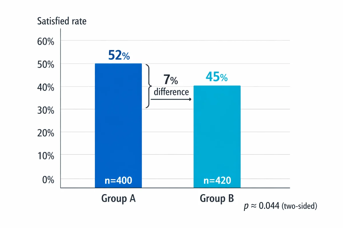
| Group | n | Satisfied | Rate |
|---|---|---|---|
| A | 400 | 208 | 52.0% |
| B | 420 | 189 | 45.0% |
- Pooled proportion: p̂ = (208 + 189) / (400 + 420) = 397 / 820 = 0.484
- Standard error: SE = √[0.484 × 0.516 × (1/400 + 1/420)] = √[0.2498 × 0.00488] = √0.001219 = 0.0349
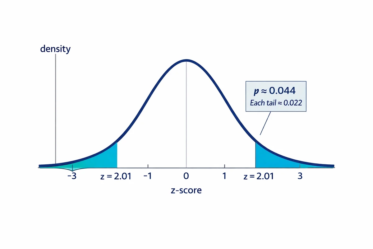
- z-statistic: z = (0.52 - 0.45) / 0.0349 = 0.07 / 0.0349 = 2.01
- p-value: For a two-tailed test, z = 2.01 gives p = 0.044
- Decision: 0.044 < 0.05 (alpha), so the 7-point difference is statistically significant at the 5% level.
Two-sample t-test (comparing means)
Use this when comparing average scores (e.g., mean satisfaction rating on a 1-5 scale).
Formula:
t = (x̄1 - x̄2) / √[ s12/n1 + s22/n2 ]
where x̄ = sample mean, s = sample standard deviation, n = sample size
The resulting t-value is compared to the t-distribution with the appropriate degrees of freedom to obtain a p-value.
Which test should I use?
| Data type | Example | Comparison | Test |
|---|---|---|---|
| Proportion (percent) | % "Satisfied" | Two groups | Two-proportion z-test or chi-square |
| Mean (continuous) | Average 1-5 rating | Two groups | Two-sample t-test |
| Mean (continuous) | Average 1-5 rating | 3+ groups | ANOVA (then post-hoc tests) |
| Paired data | Same people pre/post | Before vs after | Paired t-test or McNemar test |
| Two categorical variables | Role vs attrition intent | Association | Chi-square test of independence |
| Two continuous variables | Study hours vs exam score | Correlation | Pearson r with t-test |
In practice, most researchers use statistical software (R, Python, SPSS, Excel) or an online calculator rather than computing by hand. The formulas above show the underlying logic so you understand what the software is doing.
Try it: two-proportion significance calculator
Statistical vs practical significance
Statistical significance tells you whether an effect is detectable. Practical significance tells you whether the effect is large enough to matter.
A large sample can make even a trivial difference statistically significant. The IQ example from earlier illustrates this: a 2-point difference between groups is statistically significant at n = 1,000 (p = 0.001), but a 2-point IQ gap has no practical meaning for any real-world decision.
This is why researchers are increasingly encouraged to report effect size alongside p-values.
Effect size measures
Effect size quantifies the magnitude of a difference or relationship, independent of sample size.
- Cohen's d (for comparing two means): d = (mean1 - mean2) / pooled standard deviation. Rules of thumb: 0.2 = small, 0.5 = medium, 0.8 = large.
- Absolute difference (for proportions): e.g., "+7 percentage points satisfied." Simple and easy to communicate.
- Correlation coefficient r (for relationships): ranges from -1 to +1. Rules of thumb: 0.1 = small, 0.3 = medium, 0.5 = large (Cohen, 1992).
A practical approach is to set a minimum meaningful difference before analysis. For example: "We will only act if the satisfaction gap is at least 3 percentage points." Then use significance testing to check whether the data supports a difference of at least that size, not just any nonzero gap.
- Report the estimate: show the two values (means, percentages), not just "significant."
- Report the effect size: include Cohen's d, the absolute difference, or r.
- Report uncertainty: include a confidence interval around the difference when possible.
- Connect to decisions: explain what a difference of this size means operationally.
What does "significant difference" mean in research?
A significant difference means the observed gap between two (or more) groups is unlikely to have occurred by chance alone, given the sample sizes and the chosen significance level.
For example, if a clinical trial finds that patients taking Drug A had a recovery rate of 72% vs 65% for Drug B, and a chi-square test produces p = 0.03, researchers would report a statistically significant difference at the 0.05 level. The 7-point gap is real enough that random sampling variability is an unlikely explanation.
What does "no significant difference" mean?
"No significant difference" means the test did not produce strong enough evidence to reject the null hypothesis. Critically, this is not the same as saying the groups are identical. It could mean:
- The true difference is zero (or negligibly small).
- The true difference exists but the sample was too small to detect it (low statistical power).
- The variability in the data was too large relative to the difference.
When you encounter "no significant difference" in a study, check the sample size and the width of the confidence interval before concluding the groups are equivalent.
Statistical vs everyday meaning
In everyday language, "significant" means "important" or "noteworthy." In statistics, it means only that the result is unlikely under the null hypothesis. A statistically significant difference can be trivially small (as in the 2-point IQ example), and a non-significant difference can still be practically meaningful if the study was underpowered. Always read "significant" in context.
What does "significant relationship" mean in research?
A significant relationship (or significant association) means the observed correlation between two variables is unlikely to be zero in the population. In other words, the variables appear to move together in a pattern that is not easily explained by chance.
The most common test for a significant relationship between two continuous variables uses the Pearson correlation coefficient (r) and a t-test:
t = r × √(n - 2) / √(1 - r2)
Example: A researcher measures study hours and exam scores for 50 students and finds r = 0.45. Is the relationship significant?
- t = 0.45 × √(48) / √(1 - 0.2025) = 0.45 × 6.928 / 0.893 = 3.49
- With 48 degrees of freedom, t = 3.49 gives p < 0.001.
- Since p < 0.05, the relationship is statistically significant. Study hours and exam scores are positively correlated in a way that is not explained by chance.
What does "no significant relationship" mean?
It means the data do not provide enough evidence to conclude the variables are correlated. The true correlation might be zero, or it might be weak enough that your sample could not detect it. A non-significant relationship does not prove the variables are unrelated.
Significant difference vs significant relationship
| Significant difference | Significant relationship | |
|---|---|---|
| What it tests | Whether groups differ on an outcome | Whether two variables move together |
| Typical data | One categorical variable (groups) and one outcome | Two continuous variables |
| Common tests | t-test, ANOVA, chi-square | Pearson r, Spearman rho, regression |
| Example | "Men and women differ in job satisfaction" | "Hours of training correlates with performance" |
Common mistakes and pitfalls
1) Multiple comparisons
If you run 20 tests at alpha = 0.05, you should expect about 1 "significant" result by chance even when nothing real is going on. This is the multiple comparisons problem. Solutions include the Bonferroni correction (divide alpha by the number of tests) or controlling the false discovery rate. At minimum, distinguish between pre-planned (confirmatory) and exploratory comparisons.
2) p-hacking
Running many analyses and selectively reporting the ones that reach significance inflates false-positive rates. Common forms include: testing different survey question wordings, trying different exclusion criteria, switching between one- and two-tailed tests after seeing data, and adding or removing covariates until p drops below 0.05. The fix is to define your analysis plan before looking at results.
3) Confusing significance with causation
A significant difference or relationship does not prove causation. If Group A differs from Group B, the difference could be due to a third variable (a confounder). Observational studies can show association, but causal claims require controlled experiments or careful causal-inference methods. See correlational research.
4) Ignoring sample quality
A tiny p-value can coexist with a badly biased sample. If the wrong people respond, or response rates differ systematically by group, you may get "precise" but misleading estimates. Significance does not fix response bias or poor sampling.
5) Treating "not significant" as "no effect"
"Absence of evidence is not evidence of absence." A non-significant result might reflect low power (too few observations), high variability, or a true effect that is too small to detect with the available data. Report confidence intervals to show the range of plausible effect sizes.
Applying significance tests to surveys
Surveys generate data that is well suited to significance testing: you often compare groups (segments, time periods, treatments) on measurable outcomes (satisfaction rates, NPS, average ratings). If you have not built your survey yet, start with how to make a survey and return here once you have results. Below is a practical workflow for using significance testing on survey projects.
Define the decision first
What action changes if the metric is higher or lower? Write down the minimum difference that would trigger action before you analyze.
Plan comparisons and sample size
Decide which segments and metrics to compare. Ensure each subgroup has enough n for the differences you care about (see sample size).
Field with sampling in mind
Use appropriate random sampling or recruitment controls. Track response rates by segment so you can spot nonresponse patterns early.
Clean and validate data
Run consistent exclusion rules (speeders, duplicates, ineligible respondents). Keep a short log of what was removed and why (see data quality).
Run the right test
Use the test selection table above. For proportions: two-proportion z-test. For means: t-test (two groups) or ANOVA (3+ groups). For relationships: Pearson r or regression.
Report: estimate, uncertainty, meaning
Write one sentence that includes the two values, the difference, and the p-value, plus one sentence on practical meaning. Use research best practices to keep reporting consistent.
Example survey report language:
- Good: "Group A reported 52% satisfied vs 45% in Group B (7-point gap; z = 2.01, p = 0.044)."
- Avoid: "The segments are significantly different" (too vague) or "We proved A is better" (too strong).
Verify you are comparing like with like: same question wording, same scale labels, same field period, and comparable respondent eligibility rules. Otherwise you are testing a mix of real differences and measurement artifacts.
References
- Centers for Disease Control and Prevention, National Center for Health Statistics. (n.d.). Statistical significance. In Health, United States: Sources and Definitions.
- National Institutes of Health, National Center for Advancing Translational Sciences. (n.d.). Statistical significance. NCATS Toolkit (Glossary).
- U.S. Department of Education, NCES. (n.d.). Statistical significance and sample size. National Assessment of Educational Progress (NAEP).
- Cox, D. R. (2020). Statistical significance. Annual Review of Statistics and Its Application, 7, 1-10.
- Wasserstein, R. L. & Lazar, N. A. (2016). The ASA statement on statistical significance and p-values. The American Statistician, 70(2), 129-133.
- Wasserstein, R. L., Schirm, A. L. & Lazar, N. A. (2019). Moving to a world beyond "p < 0.05." The American Statistician, 73(sup1), 1-19.
- Cohen, J. (1992). A power primer. Psychological Bulletin, 112(1), 155-159.
- Fisher, R. A. (1925). Statistical Methods for Research Workers. Oliver & Boyd.
- Benjamin, D. J. et al. (2018). Redefine statistical significance. Nature Human Behaviour, 2, 6-10.
- Moore, D. S., McCabe, G. P. & Craig, B. A. (2021). Introduction to the Practice of Statistics (10th ed.). W. H. Freeman.
- Creswell, J. W. & Creswell, J. D. (2023). Research Design: Qualitative, Quantitative, and Mixed Methods Approaches (6th ed.). SAGE Publications.
Frequently Asked Questions
Does p < 0.05 mean there is a 95% chance the result is true?
No. A p-value is computed assuming the null hypothesis is true. p < 0.05 means your observed data (or more extreme data) would be uncommon under the null model, not that your conclusion has a 95% probability of being true.
If a result is not significant, does that mean there is no difference?
Not necessarily. "Not significant" usually means you do not have enough evidence (given your sample size and variability) to rule out chance. The true difference could be small, or your sample could be too small to detect it.
Should I always use alpha = 0.05?
No. 0.05 is a convention, not a law. Use a stricter threshold (like 0.01) when false positives are costly or when you are running many comparisons. Let the consequences of a wrong decision guide your choice.
Why did a tiny difference become significant after I got more responses?
Because bigger samples reduce random error. With enough data, even very small effects produce small p-values. That is why you should always pair p-values with effect size and a minimum meaningful difference.
Can I use significance tests on Likert-scale survey questions?
Often, yes. Teams commonly compare mean scores with a t-test (two groups) or ANOVA (3+ groups), especially with 5- or 7-point scales and moderate sample sizes. You can also compare top-box percentages using a proportions test.
What is a statistically significant p-value?
A p-value is considered statistically significant when it falls below your chosen alpha level. The most common threshold is p < 0.05, but fields differ: clinical trials often require p < 0.01, and particle physics uses the equivalent of p < 0.0000003 (5 sigma).
What does "no significant difference" mean?
"No significant difference" means the data did not provide enough evidence to reject the null hypothesis at your chosen alpha level. It does not prove the groups are identical. The difference might be too small for your sample to detect, or you might need more data.
What is considered statistically significant?
By the most common convention, a result is statistically significant when p < 0.05 (a 5% significance level). But the threshold depends on context. Genomics often requires p < 5 x 10^-8, while exploratory business analyses sometimes accept p < 0.10.
What does it mean for findings to be statistically significant?
It means the observed result would be unlikely to occur by random chance alone if there were truly no effect or no difference. It signals that the data are inconsistent with the null hypothesis at the chosen significance level.
What is the difference between a significant difference and a significant relationship?
A significant difference means two or more groups differ on some measure (e.g., Group A scored higher than Group B). A significant relationship means two continuous variables move together (e.g., hours studied correlates with exam score). Both are tested with hypothesis tests and p-values, but they answer different questions.
How do you know if results are statistically significant?
Run an appropriate statistical test for your data type, obtain a p-value, and compare it to your chosen alpha level. If p is less than alpha (commonly 0.05), the result is statistically significant.
What number is statistically significant?
There is no single number that is "statistically significant" on its own. Significance depends on the p-value relative to your alpha level. The most common rule of thumb is p < 0.05, but the appropriate threshold depends on the field, the consequences of error, and how many tests you are running.